Writing Custom Analysis Plugins for Synaptipy
This guide explains how to add your own analysis function to Synaptipy as a new tab in the Analyser - without modifying any Synaptipy source code. You write a single Python file, drop it in a folder, and your analysis appears in the GUI and batch engine the next time the application starts.
Table of Contents
1. Overview - How the Plugin System Works
Synaptipy has a central AnalysisRegistry - a Python class that maps named
analysis functions to the GUI and batch engine. You register a function by
decorating it with @AnalysisRegistry.register(...). The decorator stores the
function and its metadata (parameter definitions, plot overlays, label, etc.).
At startup, Synaptipy:
Loads all built-in analyses from
src/synaptipy/core/analysis/.Scans
~/.synaptipy/plugins/for your personal, downloaded, or third-party additions. Example plugins are available on demand through Help > Download Example Plugins…; source checkouts and desktop bundles may also expose an optional example directory for development/demo use. If a file with the same stem name exists in both places, the user copy takes precedence and a warning is written to the log.Builds the Analyser GUI. For every registered analysis that does not already have a hand-coded tab class, a metadata-driven tab is created automatically - complete with parameter widgets, a Run button, a results table, and plot overlays. Your function appears as a new sub-tab.
┌──────────────────────────────────────────────────────────┐
│  ~/.synaptipy/plugins/synaptic_charge.py                 │
│                                                          │
│  @AnalysisRegistry.register(                             │
│      name="synaptic_charge",                             │
│      label="Synaptic Charge (AUC)",                      │
│      ui_params=[...],                                    │
│      plots=[...]                                         │
│  )                                                       │
│  def run_auc(data, time, sampling_rate, **kwargs):        │
│      ...                                                 │
│      return {"module_used": "synaptic_charge",           │
│              "metrics": {"Charge_pC": 1.23,              │
│                          "Baseline_pA": -42.0}}          │
└──────────────────────────────────────────────────────────┘
         │
         ▼ startup → PluginManager.load_plugins()
┌──────────────────────────────────────────────────────────┐
│  AnalysisRegistry                                        │
│  ├── rmp_analysis          (built-in)                    │
│  ├── spike_detection       (built-in)                    │
│  ├── ...                                                 │
│  └── synaptic_charge       ← YOUR PLUGIN                 │
└──────────────────────────────────────────────────────────┘
         │
         ▼ GUI build → auto-generated MetadataDrivenAnalysisTab
┌──────────────────────────────────────────────────────────┐
│  Analyser Tab:  ... | Baseline | Spikes |                │
│                     Synaptic Charge (AUC) ◄───────────  │
│  ┌────────────────────────────────────────────┐          │
│  │ Baseline Start (s):    [0.0        ]       │          │
│  │ Baseline End (s):      [0.05       ]       │          │
│  │ Window Start (s):      [0.05       ]       │          │
│  │ Window End (s):        [0.3        ]       │          │
│  │           [ ▶ Run Analysis ]               │          │
│  │ ──────────────────────────────────────      │          │
│  │ Results: Charge = 1.23 pC                  │          │
│  └────────────────────────────────────────────┘          │
└──────────────────────────────────────────────────────────┘
You do not need to write any GUI code. The ui_params list generates the
parameter widgets, and the plots list generates the plot overlays - all from
metadata.
2. Quick Start - Your First Plugin in 5 Minutes
Copy the template:
# macOS / Linux
cp src/synaptipy/templates/plugin_template.py ~/.synaptipy/plugins/my_analysis.py

# Windows (PowerShell)
Copy-Item src\synaptipy\templates\plugin_template.py ~\.synaptipy\plugins\my_analysis.py
The plugin directory is created automatically the first time Synaptipy runs. If it does not exist yet, create it manually:
macOS / Linux:
mkdir -p ~/.synaptipy/pluginsWindows (PowerShell):
New-Item -ItemType Directory -Force "$HOME\.synaptipy\plugins"
Where is the plugins folder?
Platform
Path
macOS / Linux
~/.synaptipy/plugins/Windows
C:\Users\<YourUsername>\.synaptipy\plugins\On Windows you can open it by typing
%USERPROFILE%\.synaptipy\pluginsin the File Explorer address bar.Open the copied file in any editor.
Rename the function, change the
name=andlabel=, adjust theui_paramsandplotslists, and write your analysis logic.(Re)start synaptipy. Your analysis appears as a new tab in the Analyser.
No pip install, no editing __init__.py, no rebuilding - just save and restart.
3. The Plugin File - Anatomy of a Custom Analysis
A plugin file has two parts:
3.1 Part 1: Pure Analysis Logic
A regular Python function with explicit typed arguments and a return value. No GUI dependencies (no PySide6, no pyqtgraph).
import numpy as np

def calculate_area_under_curve(
    data: np.ndarray,
    time: np.ndarray,
    sampling_rate: float,
    baseline_start: float,
    baseline_end: float,
    window_start: float,
    window_end: float,
) -> dict:
    """Integrate baseline-subtracted trace to obtain synaptic charge (pC)."""
    bl0 = int(np.searchsorted(time, baseline_start, side="left"))
    bl1 = int(np.searchsorted(time, baseline_end,   side="right"))
    baseline = float(np.mean(data[bl0:bl1])) if bl1 > bl0 else 0.0

    wi0 = int(np.searchsorted(time, window_start, side="left"))
    wi1 = int(np.searchsorted(time, window_end,   side="right"))
    win_t = time[wi0:wi1]
    win_d = data[wi0:wi1] - baseline

    if win_t.size < 2:
        return {"error": "Integration window too narrow"}

    charge_pc = float(np.trapezoid(win_d, win_t))
    return {
        "Charge_pC":   round(charge_pc, 6),
        "Baseline_pA": round(baseline,  4),
        "_int_x": win_t,
        "_int_y": data[wi0:wi1],
        "_base":  baseline,
    }
Rules for the logic function:
Takes explicit, typed arguments - no
**kwargs.Returns a typed result object or a plain dict.
Must handle edge cases (empty data, bad windows) gracefully.
Must not import any GUI modules.
3.2 Part 2: Registry Wrapper
A thin wrapper decorated with @AnalysisRegistry.register(...). It extracts
parameters from kwargs, calls your logic function, and returns a dict that
follows the nested output schema.
from synaptipy.core.analysis.registry import AnalysisRegistry

@AnalysisRegistry.register(
    name="synaptic_charge",              # unique internal name
    label="Synaptic Charge (AUC)",       # display name in the tab
    expects_list=False,                  # True only for multi-trial statistics
    ui_params=[...],                     # parameter widgets (see §4)
    plots=[...],                         # plot overlays (see §5)
)
def run_auc_wrapper(
    data: np.ndarray,
    time: np.ndarray,
    sampling_rate: float,
    **kwargs,
) -> dict:
    """Registry wrapper for AUC / synaptic charge analysis."""
    return calculate_area_under_curve(
        data=data,
        time=time,
        sampling_rate=sampling_rate,
        baseline_start=kwargs.get("baseline_start", 0.0),
        baseline_end=kwargs.get("baseline_end",     0.05),
        window_start=kwargs.get("window_start",     0.05),
        window_end=kwargs.get("window_end",         0.3),
    )
The wrapper signature is fixed:
def wrapper(data: np.ndarray, time: np.ndarray, sampling_rate: float, **kwargs) -> Dict[str, Any]
Parameter |
Type |
Description |
|---|---|---|
|
|
1-D voltage/current trace for the selected sweep |
|
|
1-D time array in seconds, same length as |
|
|
Sampling rate in Hz |
|
All |
3.3 Return Dict Conventions
Wrappers must return a Dict[str, Any] using the nested output schema:
{
    "module_used": "my_plugin_name",   # string identifying the source module
    "metrics": {                       # all scalar results go here
        "MyMetric1": 1.0,
        "MyMetric2": 42,
    },
    # optional private keys for plot overlays (hidden from results table):
    "_fit_curve": np.array(...),
    "_event_indices": [...],
}
The metrics dict drives the results table and batch CSV columns. Any key
in metrics appears as a column header; any value that is a number is
written to the CSV.
Convention |
Behaviour |
|---|---|
|
Identifies the source; used by the batch engine to route results to the correct CSV file. |
Keys inside |
Displayed in the results table and exported to CSV. Use plain, human-readable names. |
Keys starting with |
Hidden from the results table. Use for arrays passed to plot overlays (e.g. |
Key named |
If present, the GUI shows an error message instead of results. |
Numeric values in |
Displayed as-is in the results table. |
|
Displayed as shape summary (e.g. |
|
Displayed as |
[!NOTE] Custom plugins vs. core module return types. Custom plugins must return a flat
dictas described above so the batch exporter and results table can process them generically. However, the five built-in analysis modules (passive_properties,single_spike,firing_dynamics,synaptic_events,evoked_responses) return strongly-typed Python dataclasses internally (SingleSpikeResult,TrainDynamicsResult,RinResult, etc.). If you are writing code that calls a built-in analysis function directly—rather than through the registry wrapper—access results via named dataclass attributes (e.g.result.rin_mohm) rather than dict key access. The registry wrappers translate these dataclasses into the flat dict format before returning them to the GUI and batch engine.
3.3 The expects_list Parameter
The expects_list keyword in @AnalysisRegistry.register(...) controls how
the batch engine delivers data to your wrapper function.
Value |
Data passed to wrapper |
When to use |
|---|---|---|
|
A single 1-D |
Almost always - single-sweep metrics (charge, peak amplitude, tau, etc.) |
|
A Python |
Only when you explicitly need trial-to-trial comparisons (jitter, variance, reliability) |
Why this matters in batch mode: when the batch scope is "all_trials" and
expects_list=False, the batch engine automatically averages all trials into a
single array before calling your function. This prevents
TRIAL_LENGTH_MISMATCH errors in recordings where different sweeps have
slightly different lengths (e.g. ABF files with truncated last sweeps).
# Plugin that needs a list of trials (jitter / variance calculation)
@AnalysisRegistry.register(
    name="latency_jitter",
    label="Latency Jitter",
    expects_list=True,     # <-- batch engine passes list[np.ndarray]
    ui_params=[...],
)
def run_jitter(data, time, sampling_rate, **kwargs):
    # data is a list of 1-D arrays, one per trial
    latencies = [find_first_spike(d, ...) for d in data]
    return {"module_used": "latency_jitter", "metrics": {"Jitter_ms": np.std(latencies)}}


# Plugin that operates on a single trace (most plugins)
@AnalysisRegistry.register(
    name="synaptic_charge",
    label="Synaptic Charge (AUC)",
    expects_list=False,    # <-- batch engine pre-averages if needed (default)
    ui_params=[...],
)
def run_charge(data, time, sampling_rate, **kwargs):
    # data is a single 1-D array
    return calculate_area_under_curve(data, time, ...)
4. Defining GUI Parameters (ui_params)
The ui_params list in @AnalysisRegistry.register(...) defines the parameter
widgets that appear in your tab. Each entry is a dict describing one widget.
4.1 float Parameter
Creates a double-precision spin box.
{
    "name": "threshold",          # kwarg name passed to your wrapper
    "label": "Threshold (mV):",   # label text shown in the GUI
    "type": "float",
    "default": -20.0,             # initial value (default: 0.0)
    "min": -200.0,                # minimum allowed (default: -1e9)
    "max": 200.0,                 # maximum allowed (default: 1e9)
    "decimals": 2,                # decimal places (default: 4)
    "step": 0.5,                  # step increment (optional)
}
4.2 int Parameter
Creates an integer spin box.
{
    "name": "min_spikes",
    "label": "Min Spikes:",
    "type": "int",
    "default": 3,
    "min": 1,
    "max": 10000,
}
4.3 choice / combo Parameter
Creates a drop-down combo box.
{
    "name": "direction",
    "label": "Detection Direction:",
    "type": "choice",             # "combo" also works
    "choices": ["negative", "positive", "both"],
    "default": "negative",        # pre-selected option
}
Note: You can use
"options"instead of"choices"- both keys are accepted.
4.4 bool Parameter
Creates a check box.
{
    "name": "auto_detect",
    "label": "Auto-Detect Baseline",
    "type": "bool",
    "default": False,
}
4.5 string Parameter
Creates a plain text entry field (QLineEdit). Use this for free-form strings
such as user labels or non-path text values.
{
    "name": "cell_label",
    "label": "Cell Label:",
    "type": "string",           # aliases: "str", "path"
    "default": "",
    "placeholder": "e.g. CA1 pyramidal",
    "tooltip": "Optional label stored in the results table.",
}
4.8 Common Optional Fields
These fields work on any parameter type:
Field |
Type |
Description |
|---|---|---|
|
|
Tooltip text shown on hover. |
|
|
If |
|
|
Conditional visibility - see below. |
4.9 Conditional Visibility (visible_when)
Show or hide a parameter widget based on the current value of another widget.
Example: Show "spike_threshold" only when "event_type" is set to
"Spikes":
ui_params=[
    {"name": "event_type", "type": "choice", "choices": ["Spikes", "EPSCs"],
     "label": "Event Type:", "default": "Spikes"},

    {"name": "spike_threshold", "type": "float", "default": -20.0,
     "label": "Spike Threshold (mV):",
     "visible_when": {"param": "event_type", "value": "Spikes"}},

    {"name": "epsc_threshold", "type": "float", "default": -5.0,
     "label": "EPSC Threshold (pA):",
     "visible_when": {"param": "event_type", "value": "EPSCs"}},
]
The "param" key names the sibling widget; "value" is the value that makes
this widget visible. When the controlling widget changes, visibility updates
automatically.
There is also a "context" form for clamp-mode-aware parameters:
"visible_when": {"context": "clamp_mode", "value": "current_clamp"}
5. Defining Plot Overlays (plots)
The plots list in @AnalysisRegistry.register(...) defines visual overlays
rendered on the data trace after analysis completes. Each entry is a dict.
5.1 hlines - Horizontal Lines
Draw horizontal lines at y-positions taken from the result dict.
{"type": "hlines", "data": ["threshold"], "color": "r", "styles": ["dash"]}
{"type": "hlines", "data": ["mean", "mean_plus_sd", "mean_minus_sd"],
 "color": "b", "styles": ["solid", "dash", "dash"]}
Field |
Description |
|---|---|
|
List of result-dict keys. Each key’s value → one horizontal line. |
|
Line colour (default |
|
List of |
5.2 vlines - Vertical Lines
Draw vertical lines at x-positions.
{"type": "vlines", "data": "stimulus_times", "color": "c"}
Field |
Description |
|---|---|
|
Result-dict key holding a scalar or array of x-positions. |
|
Line colour (default |
5.3 markers - Scatter Points
Draw scatter points at (x, y) positions from result arrays.
{"type": "markers", "x": "peak_times", "y": "peak_values", "color": "r"}
5.4 interactive_region - Draggable Region
A shaded region linked to two float spinboxes. Dragging the region updates the spinbox values, and changing a spinbox moves the region.
{"type": "interactive_region", "data": ["window_start", "window_end"], "color": "g"}
"data" must be a 2-element list of ui_params names (not result keys).
5.5 threshold_line - Draggable Threshold
A horizontal line synced to a float parameter widget.
{"type": "threshold_line", "param": "threshold"}
5.6 overlay_fit - Curve Overlay
Overlay a fitted curve on the trace.
{
    "type": "overlay_fit",
    "x": "_fit_time",           # result key (use _ prefix to hide from table)
    "y": "_fit_values",
    "color": "r",
    "width": 2,
    "label": "Exponential Fit",
}
5.7 popup_xy - Popup Scatter/Line Plot
Open a separate window showing e.g. an I-V or F-I curve.
{
    "type": "popup_xy",
    "title": "F-I Curve",
    "x": "current_steps_pa",
    "y": "firing_rates_hz",
    "x_label": "Current (pA)",
    "y_label": "Firing Rate (Hz)",
}
Optionally add "slope_key" and "intercept_key" for a regression line.
5.8 brackets - Burst/Event Brackets
Draw bracket bars above burst groups.
{"type": "brackets", "data": "bursts", "color": "r"}
"data" key should hold a list of arrays (each array = spike times within one
burst).
5.9 event_markers - Interactive Event Points
Scatter plot with click-to-remove and Ctrl+click-to-add.
{"type": "event_markers"}
Reads result["event_indices"] automatically.
5.10 trace - Base Trace with Overlay
Plot the trace with optional spike/event markers.
{"type": "trace", "show_spikes": True}
5.11 fill_between - Shaded Region Between Two Curves
Draw a translucent filled area between a primary curve (y1) and a baseline
curve or constant (y2). This is ideal for visualising integrated areas such
as synaptic charge transfer.
{
    "type": "fill_between",
    "x": "_int_x",        # key for the shared time array
    "y1": "_int_y",       # key for the upper/primary curve (required)
    "y2": "_base",        # key for the lower curve or scalar baseline (default: 0.0)
    "brush": (0, 100, 255, 100),  # RGBA fill colour (optional)
}
The named keys are looked up first in the top-level result dict and then inside
the nested result["metrics"] dict, so both a flat schema and the standard
{"module_used": ..., "metrics": {...}} schema are supported transparently.
y2 may be:
a key pointing to an array of the same length as
y1(arbitrary curve),a key pointing to a scalar (constant horizontal baseline), or
omitted entirely (defaults to zero).
Example - Synaptic Charge Transfer with shaded integral:
plots=[
    {"type": "interactive_region", "data": ["window_start", "window_end"], "color": "g"},
    {
        "type": "fill_between",
        "x": "_int_x",
        "y1": "_int_y",
        "y2": "_base",
        "brush": (0, 100, 255, 100),
    },
]
The corresponding return dict must include _int_x, _int_y, and _base as
private (hidden) keys:
return {
    "module_used": "synaptic_charge",
    "metrics": {"Total_Charge_pC": charge},
    "Total_Charge_pC": charge,
    "_int_x": win_time.tolist(),
    "_int_y": win_data.tolist(),
    "_base": baseline_mean,
}
5.12 trace_overlay - Highlight a Region on the Raw Trace
Draw a semi-transparent coloured segment directly on top of the raw trace to highlight an analysed time window (e.g. a baseline region or a response integration window).
{
    "type": "trace_overlay",
    "start_time": "_baseline_start_s",   # result key for start time (s)
    "end_time": "_baseline_end_s",       # result key for end time (s)
    "color": "#00cfff",                  # hex or name (default from preferences)
    "width": 3,                          # pen width in pixels
    "opacity": 60,                       # 0-100%; 100 = fully opaque
}
Field |
Type |
Description |
|---|---|---|
|
str or float |
Result key or literal float giving the region start (s). |
|
str or float |
Result key or literal float giving the region end (s). |
|
str |
Colour string or hex code. Falls back to the Trace Overlay preference if omitted. |
|
int |
Pen width (pixels, default 3). |
|
int |
0-100 (default 60). Can be overridden by the user via Plot Preferences > Trace Overlay. |
The overlay only renders when the time region lies within the currently plotted
time axis, and uses self._current_plot_data to obtain the raw trace samples.
5.13 event_fit_overlay - Overlay Fitted Event Decay Curves
Plot fitted curves (e.g. bi-exponential EPSP decays) hugging each detected event on the raw trace. Supports both single-event (1-D arrays) and multi-event (list of arrays) data.
{
    "type": "event_fit_overlay",
    "times_key": "_event_fit_times",    # result key for fit time array(s)
    "values_key": "_event_fit_values",  # result key for fit value array(s)
    "color": "#ff9900",                 # amber by default
    "width": 2,
    "opacity": 80,
}
Field |
Type |
Description |
|---|---|---|
|
str |
Result key for fit time array (1-D |
|
str |
Result key for fit value array or list of arrays. |
|
str |
Colour (falls back to Event Fit Overlay preference). |
|
int |
Pen width (default 2). |
|
int |
0-100 (default 80). |
Example return dict for an N-pulse PPR decay fit:
return {
    "module_used": "evoked_responses",
    "metrics": {
        "decay_tau_ms_p1": tau_p1,
        "decay_tau_ms_p2": tau_p2,
        # List of arrays (one per pulse) for multi-event overlay:
        "_ppr_fit_times": [t_arr_p1.tolist(), t_arr_p2.tolist()],
        "_ppr_fit_values": [v_arr_p1.tolist(), v_arr_p2.tolist()],
    },
}
The user can customise both overlay types via Edit > Plot Preferences > Trace Overlay and Event Fit Overlay tabs.
6. Where to Put Your Plugin File
Prerequisite - Enable Custom Plugins: Before your plugin will load you must ensure the “Enable Custom Plugins” checkbox is checked in Edit > Preferences > Extensions. This setting is on by default. Changes take effect immediately via hot-reload; no restart is required.
Real-world templates in examples/plugins/
Looking for a working starting point? The
examples/plugins/directory ships five fully annotated, copy-pasteable plugin templates that cover the most common use cases:
File
What it demonstrates
synaptic_charge.pyBaseline subtraction, trapezoidal integration,
fill_between+ star overlays
opto_jitter.pyMulti-channel access (TTL + voltage), per-trial loop, jitter statistics
ap_repolarization.pyDerivative-based detection,
vlines+hlinesoverlays
miniml_integration.pyDeep-learning event detection via miniML (optional dep)
spike_interface_integration.pySpike detection via SpikeInterface (optional dep)
Copy any file to
~/.synaptipy/plugins/, rename the function and thename=/label=fields in the decorator, and you have a working plugin in minutes – no blank-page problem.
Option A: Downloadable Examples Directory
Download ready-to-run example plugins using Help → Download Example
Plugins…. They are saved in ~/.synaptipy/plugins/, where you can try them
immediately and use them as templates. Enable them via Edit > Preferences
(or Synaptipy > Preferences on macOS) by checking Enable Custom Plugins;
no restart is needed.
Included Example Plugins
File |
Label in GUI |
Purpose |
|---|---|---|
|
Synaptic Charge (AUC) |
Integrates a postsynaptic current trace over a user-defined window to compute total charge (pC) via the trapezoidal rule; highlights the integrated area with a shaded fill overlay and marks the peak amplitude with a star symbol. |
|
Opto Latency Jitter |
Detects the first spike in each sweep following a TTL pulse and reports trial-to-trial latency variability (jitter) for optogenetic monosynaptic verification. Requires a secondary digital/TTL channel. |
|
AP Repolarization Rate |
Finds the steepest falling slope (dV/dt minimum) of the first action potential in a window, quantifying maximum repolarization rate in V/s as a proxy for potassium-channel dynamics. |
To use these plugins:
Choose Help → Download Example Plugins….
Open Edit > Preferences (or Synaptipy > Preferences on macOS).
Check Enable Custom Plugins. Each plugin appears as a new sub-tab in the Analyser.
To customise one, edit its file in ~/.synaptipy/plugins/. Synaptipy asks for
consent before reloading changed plugin code.
Option B: User Plugin Directory (recommended for personal additions)
Platform |
Full path |
|---|---|
macOS / Linux |
|
Windows |
|
No Synaptipy source changes needed.
File is auto-discovered at startup.
Works for any number of
.pyfiles.Will not be overwritten by upgrades.
On Windows, open the folder with
%USERPROFILE%\.synaptipy\pluginsin Explorer.
Option C: Built-in Module (for core contributors)
If you are contributing to the Synaptipy repository itself:
Create your module in
src/synaptipy/core/analysis/my_analysis.py.Add the import to
src/synaptipy/core/analysis/__init__.py:from . import my_analysis # noqa: F401 - registers: my_analysis_name
(Optional) Create a custom tab class in
src/synaptipy/application/gui/analysis_tabs/if you need GUI behaviour beyond what the metadata-driven tab provides.Add a test in
tests/core/test_my_analysis.py.
Important: The
__init__.pyimport is required. Without it, the@AnalysisRegistry.registerdecorator never executes and your analysis will not appear (see the developer guide’s Registry import rule).
7. For Core Contributors - Adding a Built-in Analysis
Step-by-step:
Step |
File |
What to do |
|---|---|---|
1 |
|
Write pure logic + registry wrapper (see §3) |
2 |
|
Add |
3 |
|
Write pytest tests for the pure logic function |
4 |
|
Add your |
Do not create a custom tab class unless you need interactive GUI features (e.g. click-to-add events, drag-to-select spikes) that the metadata-driven tab cannot provide.
8. Testing Your Plugin
Unit-testing the logic function
Since the logic function is pure Python + NumPy, test it directly with pytest:
# test_my_auc.py
import numpy as np
from my_analysis import calculate_area_under_curve

def test_auc_basic():
    fs = 10000.0
    t = np.arange(0, 0.5, 1 / fs)
    # Flat baseline followed by a rectangular current pulse
    data = np.zeros_like(t)
    data[(t >= 0.1) & (t < 0.3)] = -100.0  # 100 pA inward current, 200 ms

    result = calculate_area_under_curve(data, t, fs,
                                        baseline_start=0.0, baseline_end=0.05,
                                        window_start=0.1,   window_end=0.3)
    # Expected charge: -100 pA * 0.2 s = -20 pC (trapezoid should be close)
    assert abs(result["Charge_pC"] - (-20.0)) < 0.01
    assert result["Baseline_pA"] == 0.0

def test_auc_error_on_narrow_window():
    fs = 1000.0
    t = np.array([0.0, 0.001])
    data = np.array([0.0, -1.0])
    result = calculate_area_under_curve(data, t, fs,
                                        baseline_start=0.0, baseline_end=0.001,
                                        window_start=0.5,   window_end=0.6)
    assert "error" in result
Integration-testing the registry wrapper
import numpy as np
from synaptipy.core.analysis.registry import AnalysisRegistry

def test_auc_registered():
    # Ensure the plugin is loaded
    from synaptipy.application.plugin_manager import PluginManager
    PluginManager.load_plugins()

    func = AnalysisRegistry.get_function("synaptic_charge")
    assert func is not None

    meta = AnalysisRegistry.get_metadata("synaptic_charge")
    assert "ui_params" in meta
    assert meta.get("label") == "Synaptic Charge (AUC)"
Testing the template shipped with Synaptipy
The repository includes a test that validates the plugin template itself:
conda run -n synaptipy python -m pytest tests/core/test_plugin_template.py -v
9. Full Annotated Example - Synaptic Charge Transfer
This example measures the total synaptic charge (\(Q\), in picocoulombs) delivered during a postsynaptic current by integrating the current trace inside a user-defined time window using the trapezoidal rule.
For a current trace in pA and time in seconds the result is in pA·s = pC.
Save this as ~/.synaptipy/plugins/synaptic_charge.py (or copy it from
examples/plugins/):
"""
Custom Synaptipy Plugin: Synaptic Charge Transfer (Area Under Curve).

Drop this file in ~/.synaptipy/plugins/ and restart synaptipy.
A new "Synaptic Charge Transfer" tab will appear in the Analyser.
"""
import logging
from typing import Any, Dict

import numpy as np

from synaptipy.core.analysis.registry import AnalysisRegistry

log = logging.getLogger(__name__)


# ── Part 1: Pure logic ─────────────────────────────────────────────
def calculate_synaptic_charge(
    data: np.ndarray,
    time: np.ndarray,
    sampling_rate: float,
    window_start: float,
    window_end: float,
    baseline_start: float,
    baseline_end: float,
) -> Dict[str, Any]:
    """
    Integrate the baseline-subtracted current trace to obtain total charge.

    Args:
        data: 1-D current trace in pA.
        time: 1-D time array in seconds, same length as data.
        sampling_rate: Sampling rate in Hz.
        window_start: Start of the integration window (seconds).
        window_end: End of the integration window (seconds).
        baseline_start: Start of the baseline window (seconds).
        baseline_end: End of the baseline window (seconds).

    Returns:
        Dict with 'Total_Charge_pC' and hidden keys for plot overlays.
        Returns {'error': ...} on invalid input.
    """
    if data.size == 0:
        return {"error": "Empty data array"}

    # Baseline window
    bl_i0 = int(np.searchsorted(time, baseline_start, side="left"))
    bl_i1 = int(np.searchsorted(time, baseline_end, side="right"))
    baseline_seg = data[bl_i0:bl_i1]
    if baseline_seg.size < 2:
        return {"error": "Baseline window too narrow (need >= 2 samples)"}
    baseline_mean = float(np.mean(baseline_seg))

    # Integration window
    win_i0 = int(np.searchsorted(time, window_start, side="left"))
    win_i1 = int(np.searchsorted(time, window_end, side="right"))
    win_time = time[win_i0:win_i1]
    win_data = data[win_i0:win_i1] - baseline_mean

    if win_data.size < 2:
        return {"error": "Integration window too narrow (need >= 2 samples)"}

    # np.trapz integrates pA * s = pC
    charge_pC = float(np.trapz(win_data, win_time))

    return {
        "module_used": "synaptic_charge",
        "metrics": {
            "Total_Charge_pC": round(charge_pC, 4),
        },
        # Scalar top-level key for the results table
        "Total_Charge_pC": round(charge_pC, 4),
        "Baseline_pA": round(baseline_mean, 4),
        # Private keys for plot overlays
        "_baseline_level": baseline_mean,
        "_int_x": win_time.tolist(),
        "_int_y": (data[win_i0:win_i1]).tolist(),
        "_base": baseline_mean,
    }


# ── Part 2: Registry wrapper ──────────────────────────────────────
@AnalysisRegistry.register(
    name="synaptic_charge",
    label="Synaptic Charge Transfer",
    ui_params=[
        {
            "name": "baseline_start",
            "label": "Baseline Start (s):",
            "type": "float",
            "default": 0.0,
            "min": 0.0,
            "max": 1e9,
            "decimals": 4,
        },
        {
            "name": "baseline_end",
            "label": "Baseline End (s):",
            "type": "float",
            "default": 0.05,
            "min": 0.0,
            "max": 1e9,
            "decimals": 4,
        },
        {
            "name": "window_start",
            "label": "Integration Start (s):",
            "type": "float",
            "default": 0.05,
            "min": 0.0,
            "max": 1e9,
            "decimals": 4,
        },
        {
            "name": "window_end",
            "label": "Integration End (s):",
            "type": "float",
            "default": 0.3,
            "min": 0.0,
            "max": 1e9,
            "decimals": 4,
        },
    ],
    plots=[
        # Draggable region over the baseline window
        {"type": "interactive_region", "data": ["baseline_start", "baseline_end"], "color": "b"},
        # Draggable region over the integration window
        {"type": "interactive_region", "data": ["window_start", "window_end"], "color": "g"},
        # Horizontal line at the baseline level
        {"type": "hlines", "data": ["_baseline_level"], "color": "b", "styles": ["dash"]},
        # Shaded fill between the raw current and the baseline level
        {
            "type": "fill_between",
            "x": "_int_x",
            "y1": "_int_y",
            "y2": "_base",
            "brush": (0, 100, 255, 100),
        },
    ],
)
def run_synaptic_charge_wrapper(
    data: np.ndarray,
    time: np.ndarray,
    sampling_rate: float,
    **kwargs,
) -> Dict[str, Any]:
    """Registry wrapper - extracts kwargs and calls pure logic."""
    return calculate_synaptic_charge(
        data=data,
        time=time,
        sampling_rate=sampling_rate,
        window_start=kwargs.get("window_start", 0.05),
        window_end=kwargs.get("window_end", 0.3),
        baseline_start=kwargs.get("baseline_start", 0.0),
        baseline_end=kwargs.get("baseline_end", 0.05),
    )
The key design points illustrated here:
A dedicated baseline window is used to subtract the holding current before integration, keeping the result physically meaningful.
np.trapzis used for trapezoidal integration (not a simple sum), which is exact for linear interpolations between sample points.The return dict follows the nested output schema
{"module_used": ..., "metrics": {...}}alongside flat scalar keys for the results table.Two
interactive_regionoverlays let the user drag both windows directly on the trace without typing numbers.A
fill_betweenoverlay shades the integrated area, making the charge visually obvious on the trace._baseline_level,_int_x,_int_y, and_base(private keys) feed the plot overlays without appearing in the results table.
10. Applying Global Themes to Plugins
Synaptipy ships a global plot-customisation system (shared/plot_customization.py)
that lets users change trace colours, line widths, scatter sizes, and region
fills from Edit > Preferences > Plot Customisation. When a user saves new
preferences, a preferences_updated signal fires and all built-in canvases
instantly re-style their existing plot items - no file reload required.
How the theme reaches your plugin
The registry wrapper receives all GUI state through **kwargs. Synaptipy
injects a theme_config dict whenever the current plot-customisation settings
are relevant to the analysis call. Your wrapper can read it like this:
@AnalysisRegistry.register(name="my_metric", ...)
def run_my_metric_wrapper(data, time, sampling_rate, **kwargs):
    theme_config = kwargs.get("theme_config", {})

    # Retrieve individual style properties with sensible defaults
    trace_color  = theme_config.get("single_trial_color", (200, 200, 200))
    avg_color    = theme_config.get("average_color",      (255, 255,   0))
    scatter_color = theme_config.get("scatter_color",     (255,   0,   0))
    line_width   = theme_config.get("line_width",         1.5)

    return my_metric_logic(data, time, sampling_rate,
                           trace_color=trace_color,
                           avg_color=avg_color)
Available keys in theme_config:
Key |
Type |
Description |
|---|---|---|
|
|
Colour of individual trial traces |
|
|
Colour of the average overlay |
|
|
Colour of scatter / event markers |
|
|
Fill colour of |
|
|
Colour of threshold |
|
|
Stroke width for all trace pens |
|
|
Symbol size for scatter plots |
Always guard with .get("key", default) so your plugin works even when
theme_config is absent (e.g. in batch-only usage or unit tests).
Returning styled plot data
If your analysis produces overlay arrays (stored under private _-prefixed
keys), you can store the chosen colour alongside them so the canvas can apply
it verbatim:
return {
    "My_Value": 42.0,
    "_plot_x": time_slice,
    "_plot_y": data_slice,
    "_plot_color": theme_config.get("average_color", (255, 255, 0)),
}
The canvas reads _plot_color when drawing the overlay curve and passes it
directly to pg.mkPen().
Listening to live theme changes in a popup window
If your plugin opens a secondary pg.PlotWidget popup (via the popup_xy
plot type), connect to the global signal so it re-styles on the fly:
from synaptipy.shared.plot_customization import get_plot_customization_signals

signals = get_plot_customization_signals()
signals.preferences_updated.connect(my_popup_widget.update_pens)
11. SpikeInterface Integration Plugin
Synaptipy ships a ready-to-use plugin that integrates
SpikeInterface spike detection
directly into the standard Analyser workflow. Because SpikeInterface is an
optional dependency it is not listed in requirements.txt; install it once
with pip install spikeinterface.
What the plugin does
You select the extracellular field channel in the Analyser tab (exactly like any other built-in analysis).
The plugin wraps the selected 1-D numpy array in a
spikeinterface.core.NumpyRecording, bandpass-filters it (default 300-6000 Hz), and runsdetect_peakswith theby_channelmethod - no external sorter binary is required.Detected spike times are shown as:
Red dashed vertical lines on the trace (one line per spike).
Red scatter markers at the filtered amplitude of each peak.
Summary metrics appear in the Results panel:
Spike_Count,Noise_Estimate,Threshold, andMean_Firing_Rate_Hz.
Before running
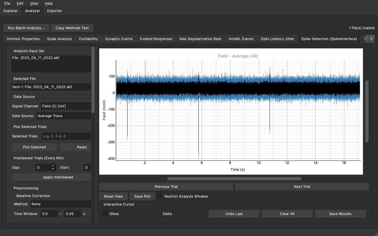
The tab renders automatically when the plugin file is present in
examples/plugins/ or ~/.synaptipy/plugins/. The Run Analysis button
(run_button=True in the decorator) means the analysis only executes when
clicked - it does not re-run on every parameter change, which is appropriate
for the relatively expensive bandpass + peak-detection pipeline.
After running - 3 detected spikes
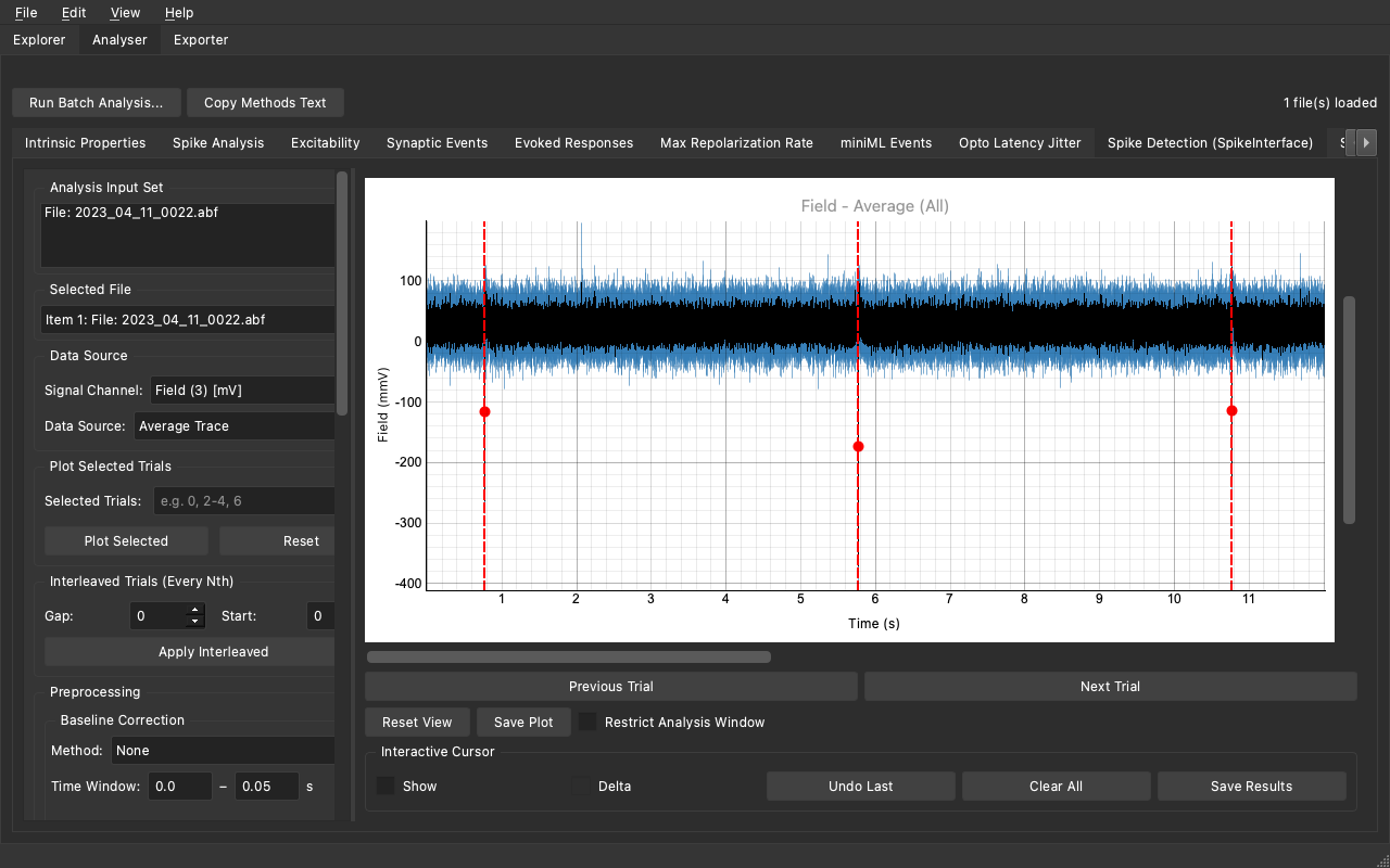
Red dashed lines mark each detected spike time; red circles mark the filtered amplitude at each peak. The Results panel shows all four metrics.
Installation
# Activate the Synaptipy environment and install SpikeInterface
conda activate synaptipy
pip install spikeinterface

# The plugin is already present at:
#   examples/plugins/spike_interface_integration.py
# Copy it to your personal directory for auto-load on every launch:
cp examples/plugins/spike_interface_integration.py ~/.synaptipy/plugins/
Key parameters
Parameter |
Default |
Description |
|---|---|---|
|
300 Hz |
Lower bandpass cutoff (removes LFP / baseline drift) |
|
6000 Hz |
Upper bandpass cutoff (removes high-frequency noise) |
|
5 |
Spike threshold as a multiple of the MAD noise estimate |
|
|
Polarity: |
|
5 ms |
Refractory period - prevents double-counting secondary deflections |
Testing the plugin without running the full CI suite
The plugin tests live in examples/tests/ and are intentionally excluded from
the core CI testpaths (which only scans tests/). Run them manually:
conda run -n synaptipy python -m pytest examples/tests/ -v
12. Deep Learning & Third-Party Integrations (e.g., miniML)
Synaptipy’s plugin architecture is intentionally decoupled from its core
dependencies. You can integrate heavy machine-learning or third-party
libraries – such as miniML, a
deep-learning framework for synaptic event detection – without modifying
any Synaptipy source files and without adding those dependencies to
requirements.txt, pyproject.toml, or environment.yml.
CI contract:
miniML,tensorflow,keras,ruptures, and any other third-party ML library must never be added to Synaptipy’s core dependency files. The CI pipelines are headless, fast, and must remain completely decoupled from these optional dependencies.
4-step workflow
Clone miniML once (outside the Synaptipy directory):
git clone https://github.com/delvendahl/miniML.git ~/miniML
miniML is not a pip package – it is a collection of Python source files. The plugin adds
miniML/core/tosys.pathat runtime.Install miniML’s Python dependencies into the Synaptipy environment:
conda activate synaptipy
pip install "tensorflow>=2.12,<2.16" scikit-learn ruptures==1.1.10
Do NOT run
pip install -r ~/miniML/requirements.txt. That file pinsnumpy==1.23.5andpandas==1.5.3, which are incompatible with Synaptipy’snumpy>=2.0requirement and will breaknp.trapezoidcalls throughout the application.Copy the plugin to your personal plugin directory:
# macOS / Linux
cp examples/plugins/miniml_integration.py ~/.synaptipy/plugins/

# Windows (PowerShell)
Copy-Item examples\plugins\miniml_integration.py ~\.synaptipy\plugins\
Enable custom plugins under Edit > Preferences (or Synaptipy > Preferences on macOS) and restart.
Use the Browse buttons in the GUI:
Open a recording, switch to the Analyser tab, click miniML Events.
Click Browse… next to miniML core/ Path and navigate to the
core/sub-directory inside the cloned repo (e.g.~/miniML/core/).Click Browse… next to Model Path (.h5) and navigate to a
.h5model file (e.g.~/miniML/models/GC_lstm_model.h5).Adjust Prediction Threshold and Direction, then click Run Analysis.
miniML Integration Example
Because Synaptipy plugins run in your local environment, you can easily
integrate heavy ML frameworks like miniML without bloating Synaptipy’s
core dependencies. We provide a template at
examples/plugins/miniml_integration.py.
Installation warning
Do NOT use pip install miniML (it targets an unrelated database package
on PyPI) and do NOT use git clone inside the Synaptipy directory (to
avoid git tracking conflicts). Install via the GitHub URL above.
Template: examples/plugins/miniml_integration.py
A fully annotated, copy-pasteable template is provided at
examples/plugins/miniml_integration.py. It demonstrates:
Lazy
sys.pathimport – the plugin adds theminiML/core/directory tosys.pathat analysis time (via_import_miniml(miniml_core_path)), so the library is never imported at Synaptipy startup. This means the tab appears even when miniML is not installed; users only see an error if they click Run Analysis without filling in the paths.dirpathBrowse button forminiml_core_path– users click Browse instead of typing a path.filepathBrowse button formodel_path– opens a file picker pre-filtered to.h5/.kerasmodel files.How to expose
threshold,direction, andbatch_sizeas GUI widgets.How to return private
_event_times/_event_peakskeys for plot overlays while keepingEvent_Count,Frequency_Hz, andModel_Usedvisible in the results table.run_button=Truein the decorator – for analyses that should only run on explicit user action (rather than on every parameter change), set this flag to add a dedicated Run Analysis button to the tab.
miniML API notes (common pitfalls)
The miniML library splits its configuration across two call sites.
Getting this wrong causes a TypeError or silent bad output.
EventDetection.__init__() parameters
Pass only these arguments to the constructor:
detector = EventDetection(
    data=trace,
    event_direction=direction,   # "negative" or "positive"
    model_path=active_model,
    model_threshold=threshold,
    batch_size=batch_size,
    window_size=window_size,
)
rel_prom_cutoff, convolve_win, and gradient_convolve_win are not
accepted by __init__() – passing them there raises a TypeError.
detect_events() parameters
All post-processing controls belong in the detect_events() call:
detector.detect_events(
    eval=True,
    rel_prom_cutoff=rel_prom_cutoff,   # default 0.25
    convolve_win=convolve_win,          # default 20
    gradient_convolve_win=gradient_convolve_win,  # default 40
)
Never pass
convolve_win=0orgradient_convolve_win=0. miniML uses these as slice offsets:smth_gradient[-0:]in Python evaluates to the entire array because-0 == 0, silently zeroing the gradient signal. With all-zero gradient,np.std([])returnsNaNin NumPy >= 2.0, causing aValueError: cannot convert float NaN to integerdeep inside miniML’s peak-finding code. Use the documented defaults (20 and 40) or any positive non-zero value.
Marker placement: onset vs. amplitude peak
detector.event_locations contains onset indices (the steepest-slope
sample), not amplitude peaks. If you plot markers directly at those indices
the dots appear shifted left relative to the visible peak.
The plugin searches forward from each onset within window_size // 2 samples
using np.argmin (negative events) or np.argmax (positive events) to find
the true peak:
half_win = max(1, window_size // 2)
find_extremum = np.argmin if direction == "negative" else np.argmax
for k, onset in enumerate(valid_locs):
    end_idx = min(int(onset) + half_win, len(data))
    seg = data[int(onset):end_idx]
    peak_indices[k] = onset + find_extremum(seg) if len(seg) > 0 else onset
Adapting the template to other ML tools
The same pattern works for any inference library:
Part |
What to change |
|---|---|
|
Replace |
|
Use whatever path or identifier your model needs |
|
Replace miniML API calls with your library’s API |
|
Expose whichever hyperparameters the user should control |
|
Map returned private keys to the overlay type that fits |
13. Troubleshooting
Symptom |
Cause |
Fix |
|---|---|---|
Tab does not appear |
Plugin file has a syntax error |
Check the Synaptipy log ( |
Tab does not appear |
File not in the plugins folder |
Verify the path: macOS/Linux: |
Tab does not appear |
Missing |
The file must contain a decorated function. |
|
Plugin imports a package not installed in your environment |
Install the dependency: |
|
Two plugins use the same |
Change one plugin’s |
Parameters don’t show up |
|
Must be one of: |
Browse button not shown |
Using |
Change type to |
miniML tab appears but shows error on Run |
|
Browse to the |
Plot overlay missing |
Result dict key doesn’t match |
The key in |
Results table shows |
Keys must start with underscore |
Prefix with |
Built-in contrib: 0 tabs on Windows |
Forgot to add |
See §7, step 2. |